Models

Below are summaries of our models, for more information please read our detailed report linked here: https://github.com/edinhluo/DSC180-Capstone-Project/blob/main/report.pdf

Non-Adaptive and Adaptive Pooling

To simulate COVID testing, a matrix-based analysis was used as the primary testing strategy. Given a matrix denoting which samples belong to a pooled test, each row representing a pooled test would contain either a 0 (the sample is not in the pool) or a 1 (the sample is in the pool). If at least 1 person in this pool is COVID positive, the output-tested vector would return a 1, indicating the entire pool contains a positive sample. Conversely, a 0 indicated a negative sample, where all samples in the group were “released” from testing as they are labeled negative and were not considered positive candidates. In the figure below, you see an example of our pool matrix, infected vector, and test vector that our simulations produce. On the top, is an initial infected vector, bottom left shows our pooling matrix, and the bottom right shows the output test vector. In a nonadaptive strategy, the pooling scheme was all done in one step, where all tests were run at the same time to determine its positive candidates. In an adaptive strategy, tests were separated in steps, where the pooling strategies in proceeding steps changed based on the prior result. In our method, an adaptive strategy follows that if a test is negative, all samples within that row are removed from the tests, while all the remaining positive candidates are tested once again but under different parameters given by the remaining sample size.

Disjoint Pooling and Limited Pool Size

To ensure that samples were equally tested amongst the simulation, disjoint pools were adapted into both the nonadaptive and adaptive strategies. Rather than randomly pick the samples at the start of each test, all samples were shuffled, then divided according to pool sizes. Given a pool size s, sample size n, and starting test number t = n / s, this guarantees that in the first t tests, every sample is tested only once and that there is no overlap between the first t tests. After all samples are run equally in the first t tests, the remaining pool (whether nonadaptive or adaptive pooling) is reshuffled and divided once again for the following t tests. Complications with our models arise from high pooling sizes because large pools above 32 samples may dilute the samples where positive COVID samples are not detectable through normal laboratory means[3]. In order for COVID to be detectable in larger pool sizes, the laboratory would require longer lengths to examine, which is even less optimal. To reflect this reality, pool sizes were limited to a maximum of 32, as positive COVID samples were detectable at this size, but were less favorable with larger sizes[3].

Degree Centrality Pooling

Classical SEIR disease model:

To create testing results based on a more-realistic real-world setting, we considered using a social network in our project. In the Degree Centrality Pooling, we use the classical SEIR disease model to simulate the real world. The SEIR model divides the population into five categories: Susceptible (S), Exposed (E), Infectious (I), and Recovered (R) or Death (D) groups (see below pic). So, there are five states of individuals in the spread of the disease: when a person is exposed to the virus, they will change from the susceptible state (S) to the exposed state (E). When the virus develops in the body for a while (incubation period), they will be infected and become a patient (I) and will either recover (R) or die (D).

The most significant difference between simulated and network data is that all simulated test data are independent: there is no connection between them. Their chances of being pooled and infected are unrelated. However, in the social network data, the infectious rate is interdependent like reality.

Degree Centrality Pooling Strategy:

We use the degree centrality to assess nodes’ importance based on their number of connections. In other words, if this node has an above-average number of connections, this node has a high degree centrality. (See below pic)

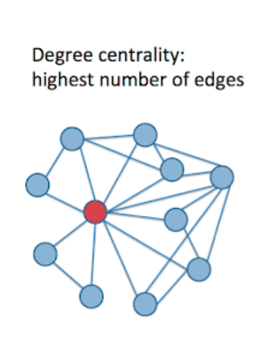
First, we sort the degree centrality of all nodes. For the top ranked nodes, we perform individual tests on them as their chance of being positive is high as they contact a lot of people. Then for above average nodes, we create multiple smaller size group pools to test them compared to the rest low degree centrality pools. In conclusion, we prioritize nodes with high degree centrality in this algorithm. The higher the degree centrality is, the more frequent the testing is and smaller the pool size is.

Tensor Based Pooling

The tensor based model is based on placing samples within the elements of a rank 2 tensor (matrix). The columns and rows represent the pools during our testing phase and will be used to create the testing matrix. After testing, all samples in unaffected pools are either retested or labeled as positive. Given that n is the number of samples to be tested, the number of samples in each pool within our tensor method will be given by (ceiling(2n))and the number of tests in each tensor run is calculated to be 2ceiling(2n).

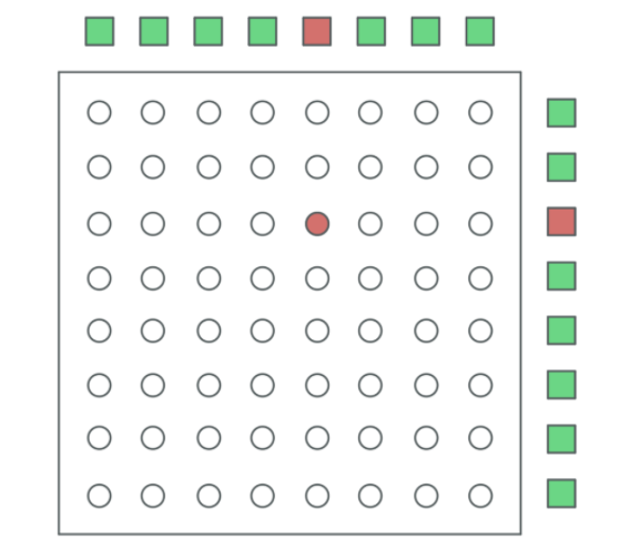
The picture above is an example of our rank 2 tensor method, in which sample 21 is in pool 5 and in pool 11.

Machine Learning Pooling

Extended-SEIR disease model:

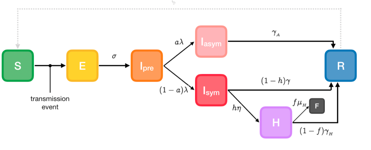
The extended-SEIRD model divided the subpopulation Infectious group (I) from the SEIR model into pre-symptomatic (Ipre), asymptomatic (Iasym), symptomatic (Isym), and hospitalized (H). This model takes into account the latent period of the virus and different transmission rates in different symptomatic stages which is similar to the real Covid-19 disease. Henceforth, there are a total eight states of individuals in the spread of the disease: when a person is exposed to the virus, they change from the susceptible state (S) to the exposed state (E). When the virus develops in the body (Ipre) for a while (incubation period), they will be infected and become a patient. However, the COVID-19 patient may develop symptoms (Isym) or not (Iasym). Symptomatic patients with severity will be hospitalized (H) and will either recover (R) or die (D). On the other hand, Mild patients will recover after a while. (See below pic)

Demographic Model:

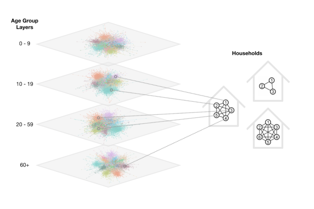
Besides the disease model, we also employ the demographic model to simulate the community level contact network. This model assigns each node to a household and to a specific age bracket. It also generates a separate out of household contact network for each age bracket. For example, there is a separate 10-19 out of household regular contact network which probably represents the secondary school community.

Machine Learning Pooling Strategy:

We extract two features from the disease network: degree centrality and eigenvector centrality. The eigenvector centrality, similar to degree centrality, assigns nodes’ importance based on the eigenvector of the network adjacency matrix. In other words, the higher the eigenvector centrality is the more connections to other high score nodes. We also use household size and age group from demographic networks. The last feature is infected count, based on Ethan’s work, which is the number of times an individual appears in a positive group test. Following picture is sample training data.

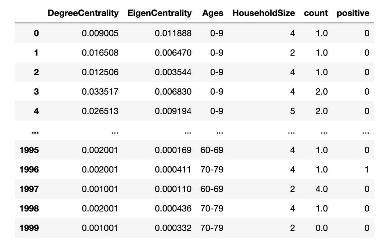
We use a balanced random forest classifier to train the model. However, there are many difficulties which force us to stop this exploratory testing work. For more details, please see result page.